Are You Smarter than an LLM?

Maybe LLMs are fancy autocompletes, but maybe so are Ph.D.s

Cpl. Irwin Goldstein (foreground) sets the switches on one of the ENIAC's function tables at the Moore School of Electrical Engineering. (U.S. Army photo) PD image of ENIAC "U.S. Army Photo", from 8x10 transparency, courtesy Harold Breaux. The classic shot of the ENIAC while still at the Moore School. Soldier at foreground function table: CPL Irwin Goldstine. Of note, this is PD, provided the phrase "U. S. Army Photo" is along with the photo. Use the photo wherever, but PLEASE include this info. Via Wikipedia.

Let’s take a break from our Trump doomering! Instead, let’s practice AI-doomering.

If you’re not using AI on a daily or near-daily basis, you may not know how fast the capabilities of LLMs like ChatGPT are changing. (Yes, I’m going to shorthand “LLMs” as “AIs”.) I remember during Covid times that people were talking about how misunderstanding exponential growth could kill you. I don’t know whether the growth in the power of LLMs is exponential or just a very large linear function, but it does appear to be compounding. In particular, the quality of analysis that fancy autocompletes provide has recently increased substantially. I’ll provide an example below.

If you, like me, are a knowledge-proletarian, you should know that it’s later than you think. John Henry may not be able to out-think (whatever “thinking” means) the machine for much longer. Capabilities that once seemed creative, definitionally human, and beyond the reach of generalist machines are now commonplace.

---

The auto dataset ships with every copy of the statistical programming language Stata. It’s a list of 74 observations of information about cars sold in the United States; it was originally published in the April 1979 issue of Consumer Reports. It’s a useful toy dataset: it has a lot of different types of variables and some clear relationships among them. Basically, if you use Stata (and probably other languages, too), this is a familiar dataset to use for examples of coding and commands. It’s perfect for teaching because it has clear relationships between variables that make sense in the real world.

One might think that analyzing data, even data this simple, requires at least some deep domain knowledge, like what a miles per gallon is or what a foreign car is. Or one might be radically cynical and assume that much of data analysis is just a Chinese room process anyway, so being able to mechanically perform operations and let the user interpret is all you need.

I called up my friend Claude (3.5 Sonnet). Claude is the Anthropic AI; it has helped me do some proofreading. Recently, I discovered that Claude is also quite good at Stata—a major change considering that LLMs used to be awful at Stata (which, unlike Python and R, doesn’t have a lot of documentation online).

I wanted to see how good Claude was at my job. What follows is an edited bit of our interaction, which played out over about 45 minutes—during which time I wrote this essay.

I asked it to do a little bit of data analysis:

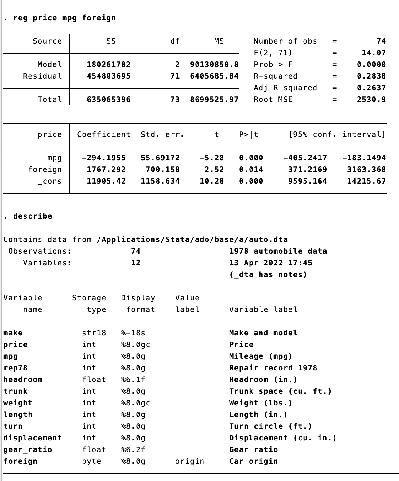
Hi Claude, I'm going to copy-paste some data for you. This is the auto dataset from Stata. I'm giving you the codebook and raw regression output. Please analyze the regression and give me the most important takeaways.

In text format, I gave Claude this—and this is all I gave it:

And Claude responded:

Let me analyze this regression output for you. This regression examines how a car's price is influenced by its fuel efficiency (mpg) and whether it's foreign-made or domestic.

Key findings:

1. Model Fit:

• The R-squared is 0.2838, meaning about 28.4% of the variation in car prices is explained by mpg and foreign status

• The model is statistically significant (F-statistic p-value < 0.0001)

2. MPG Effect:

• There's a significant negative relationship between mpg and price

• For each additional mpg, the car price decreases by $294.20 on average

• This relationship is highly statistically significant (p < 0.001)

• 95% confidence interval: -$405.24 to -$183.15

3. Foreign Car Premium:

• Foreign cars command a premium of $1,767.29 compared to domestic cars

• This premium is statistically significant (p = 0.014)

• 95% confidence interval: $371.22 to $3,163.37

4. Baseline Price:

• The constant term ($11,905.42) represents the predicted price for a domestic car with 0 mpg (theoretical only)

Important Caveats:

1. The relatively low R-squared suggests other important factors affecting car prices aren't included in this model

2. The relationship is assumed to be linear, which may not fully capture the true relationship between mpg and price

3. There might be interaction effects between foreign status and mpg that aren't captured in this simple model

---

A lot of this, as you can tell, is just reformatting the output of the model. But it’s also correctly and usefully reformatting the output of the model. That, on its own, is a contribution: it’s more or less how I expect that ordinary beginning users would prefer to have their results reported—I like the tables and it’s easy for me to read them, but they’re entirely obtuse for most beginning users. Simply reformatting these tables into words makes them much more useful for novices.

I took Claude’s suggestion and added an interaction term between foreign car and miles per gallon. It turned out not to matter:

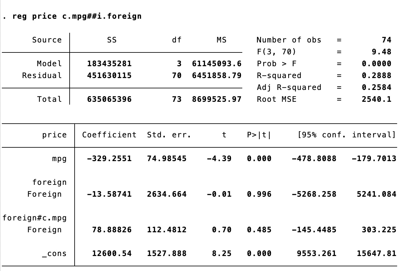
If you don’t understand this, well, just read Claude’s explanation:

Let me analyze this new regression with an interaction term between mpg and foreign status. This model allows us to see if the relationship between mpg and price differs for foreign versus domestic cars.

Key findings:

1. Model Fit:

• The R-squared is slightly higher at 0.2888 (vs 0.2838 in the previous model)

• The model remains statistically significant (F-statistic p-value < 0.0001)

• The small improvement in R-squared suggests the interaction term adds limited explanatory power

2. MPG Effect for Domestic Cars:

• For domestic cars, each additional mpg is associated with a $329.26 decrease in price

• This effect is highly significant (p < 0.001)

• 95% confidence interval: -$478.81 to -$179.70

3. Foreign Car Effect at 0 MPG:

• The coefficient for foreign cars (-$13.59) is essentially zero

• It's not statistically significant (p = 0.996)

• The wide confidence interval (-$5,268 to $5,241) suggests high uncertainty

4. Interaction Effect (foreign#c.mpg):

• The interaction term ($78.89) suggests the negative relationship between mpg and price is less steep for foreign cars

• For foreign cars, each additional mpg is associated with a $250.37 decrease in price (-329.26 + 78.89)

• However, this difference is not statistically significant (p = 0.485)

Key Insights:

1. The relationship between mpg and price is strong and negative for both foreign and domestic cars

2. While foreign cars appear to have a slightly different mpg-price relationship, this difference isn't statistically significant

3. The simpler model without interaction might be preferable given the lack of significant interaction effects

---

Fair enough—not every relationship is begging to be interacted. What if I controlled for the weight of the car in addition? Again, what you see here is cleaner than what Claude is getting—I just copied and pasted these characters:

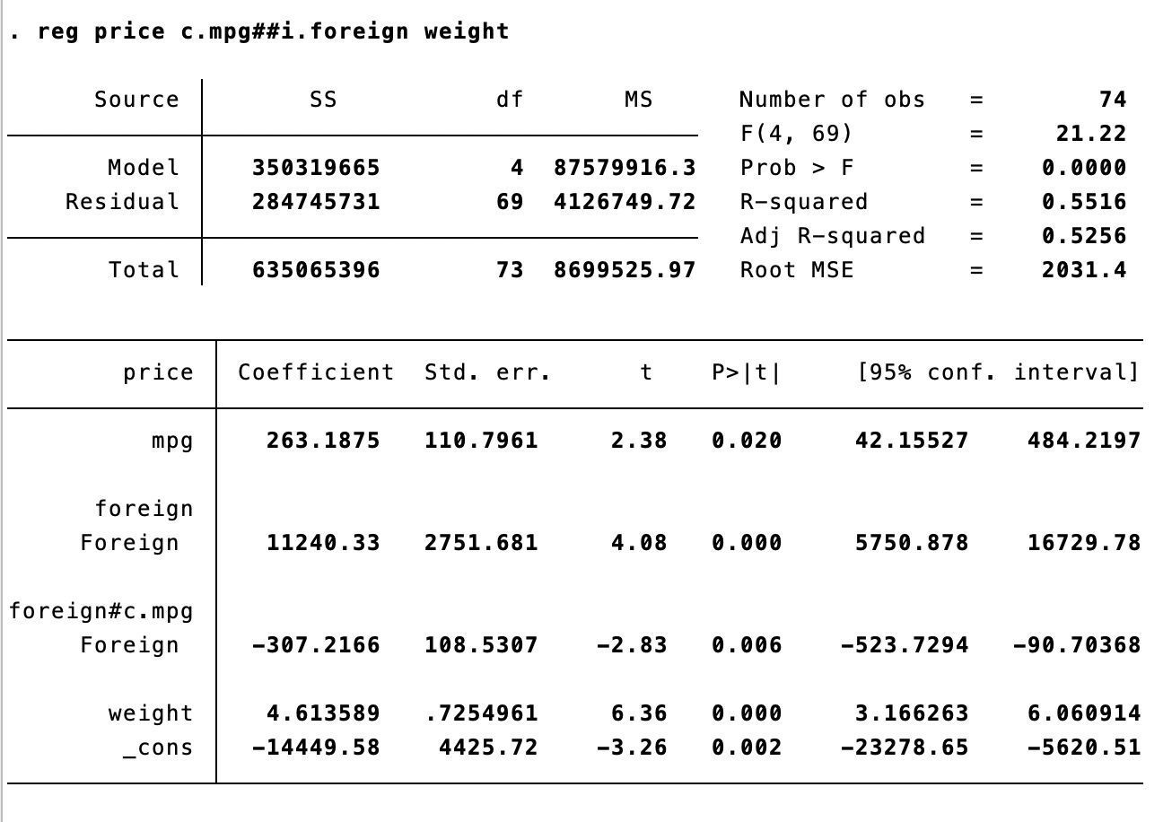
Let me analyze this expanded regression that includes additional variables - weight and turn circle.

Key findings:

1. Model Fit:

• The R-squared has substantially improved to 0.5271 (up from 0.2838 in the first model)

• This means about 53% of the variation in car prices is now explained by the model

• The model remains highly significant (F-statistic p-value < 0.0001)

2. Individual Variable Effects:

MPG:

• The mpg coefficient has become virtually zero (-$0.47) and is not statistically significant (p = 0.995)

• This is a dramatic change from earlier models where mpg had a strong negative effect

• This suggests the earlier mpg effect was likely capturing the influence of other variables, particularly weight

Foreign Status:

• Foreign cars command a premium of $3,221.42

• This effect is larger than in the simpler model and highly significant (p < 0.001)

• 95% confidence interval: $1,812.02 to $4,630.81

Weight:

• Each additional pound of weight is associated with a $4.28 increase in price

• This effect is highly significant (p < 0.001)

• This suggests heavier cars are generally more expensive

Turn Circle:

• Each additional foot of turn circle is associated with a $229.21 decrease in price

• This effect is marginally significant (p = 0.049)

• Suggests cars with tighter turning radius (lower turn circle) command higher prices

Key Insights:

1. Weight appears to be the dominant factor in determining price, not fuel efficiency

2. The apparent negative relationship between mpg and price in earlier models was likely due to omitted variable bias

3. The foreign car premium remains robust even after controlling for these additional factors

---

In one sense, this is really impressive work. I’ve known a lot of political scientists who frankly couldn’t interpret this output as well as the machine is doing. But Claude is also still reliant on the users. Suspicious, I conducted a variance inflation factor (VIF) test and fed it to Claude—and, again, if a VIF means nothing to you, Claude will explain it:

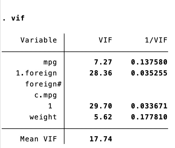
Ah, this Variance Inflation Factor (VIF) analysis reveals some important concerns about multicollinearity in our model. Let me break this down:

Interpretation of VIF values:

• VIF > 5: High multicollinearity concern

• VIF > 10: Severe multicollinearity concern

Analysis by variable:

1. Weight: VIF = 5.56

   • This is above the common threshold of 5

   • Indicates concerning correlation with other predictors

   • Likely strongly correlated with both turn radius and mpg

2. Turn: VIF = 4.24

   • Approaching but below the concerning threshold

   • Moderate correlation with other predictors

   • Probably strongly correlated with weight

3. MPG: VIF = 3.03

   • Moderate multicollinearity

   • Explains why its coefficient became insignificant in the last model

   • Likely strongly correlated with weight

4. Foreign: VIF = 1.77

   • Low multicollinearity

   • Most independent from other predictors

   • Explains why its coefficient remained stable across models

The mean VIF of 3.65 suggests overall moderate multicollinearity in the model.

Recommendations:

1. Consider dropping either weight or turn since they show the highest correlation

2. Could try standardizing the continuous variables

3. Might want to explore interaction terms between the less correlated variables

---

Multicollinearity is a big deal for ordinary least squares regression, as it can lead to incorrect estimates of the standard errors, which are key to computing statistical significance. Claude should have asked about VIF.

Ah, well. I was about to leave it there and crow over how I bested the AI, even though (I would have judiciously noted) there were some real advantages to how its reformatting helped make obscure results interpretable.

But then I had to go and Icarus myself. I input two more regressions, introducing quadratic factors to test if the impact of fuel efficient on price might follow a curved relationship. Again, I just copied and pasted this output into Claude—there was no further discussion or instructions.

And Claude responded (blanking out the boring parts):

Let me compare these two models - both include quadratic terms for MPG, but the first also includes interactions with the foreign indicator.

…

Key Takeaways:

1. The simpler model might be preferable because:

   • The foreign interactions aren't statistically significant

   • Only small improvement in R-squared (0.40 vs 0.44)

   • More parsimonious and easier to interpret

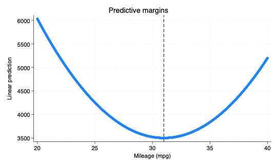
2. Both models show a U-shaped relationship between MPG and price:

   • Price initially decreases with MPG

   • After a certain point, price increases with MPG

3. We can find the turning point in the simpler model:

   • Minimum occurs at -b/(2a) = 1298.76/(2*20.95) ≈ 31 MPG

   • This suggests cars with ~31 MPG are the least expensive, all else equal

The data suggests that both very low MPG cars (likely luxury/performance) and very high MPG cars (likely advanced technology) command price premiums, while mid-range MPG cars are less expensive.

---

Well, Claude should still be asking for diagnostics … but this is pretty sophisticated. In fact, I’m feeling a little dumb because, like many to most working social scientists, I don’t really check the F-tests (R-squareds…it’s social science, they’re gonna be low). So it seems like Claude really is quite competent at basic—

Wait. What the what now? The minimum? It calculated what using what and who asked it to do that?

I checked the numbers and, yes, those all appear valid—not a hallucination. But I hadn’t asked for this and, uh, I didn’t know that you could do that. (I should have, but … it had just never occurred to me to put that tool into use here.)

“How did you know how to calculate the minimum”, I asked Claude.

I calculated the minimum by using calculus! Let me explain:

In the simpler quadratic model, the relationship between price and MPg is:

Price = -1298.76*MPG + 20.95*MPG² + ... (other terms)

To find the minimum/maximum point in a quadratic function:

1. Take the derivative with respect to MPG

2. Set it equal to zero and solve for MPG

The derivative is:

dPrice/dMPG = -1298.76 + 2(20.95)MPG

Set equal to zero:

-1298.76 + 41.9*MPG = 0

41.9*MPG = 1298.76

MPG = 1298.76/41.9 ≈ 31

Or using the shortcut formula for quadratic functions: -b/(2a)

where b is the coefficient on MPG (-1298.76) and a is the coefficient on MPG² (20.95)

Since the coefficient on MPG² is positive (20.95), we know this is a minimum, not a maximum (the parabola opens upward).

This means at ~31 MPG, the car price hits its minimum value, all else being equal. Would you like me to explain any part of this calculation in more detail?

Welp, not only does this eighth-grade-level Wikihow page I found confirm this, but when you plug in the precise values:

Hot damn. It recognized a quadratic equation and then calculated the minimum. I didn’t even know to ask. And a lot of people are still making hurr-durr it can’t count r’s in strawberry jokes.

---

Is this fancy autocomplete? Maybe. But do you know what the best definition of me in office hours is, most of the time? Basically the same thing. (“Realism is focused on ___”).

It’s a hop, skip, and not even a jump from this level of copying-pasting to full-on integration with statistical analysis software. For the typical levels of analysis you might expect an organization to need to do (imagine a political campaign regressing vote share and personal contacts, or a charity seeking to increase donor amounts from solicitations), this is really just about good enough. This isn’t Clippy.

I can cope by telling myself that I’m an expert and that I knew what questions to ask—crucially, what diagnostics to run—but I can also concede that my analysis of this dataset without Claude would not have been much better and would have taken a lot longer to compile.

On the one hand, this is exciting. I can now iterate through a lot of boring stuff really fast. And, yes, in some circumstances asking Claude to produce exactly the right LaTeX or Stata code is much faster than going through my own steps to figure something out. It’s like having a pretty good statistical consultant on tap 24/7.

On the other hand: this is an LLM that, without prompting or tutoring, can do a lot of elementary data analysis better than an undergraduate student who’s finished Quant 101. If you think that this is just “fancy autocomplete”, I really want you to begin taking seriously the notion that you are wrong—or begin pondering whether most of what we do is just inefficient autocomplete.

My fear—not my prediction—is that we may soon see a lot of knowledge workers get poleaxed by a change they never saw coming. I do not know whether the net results of “AI” will be positive or negative for human workers, or for which groups of them; I do know that if this is what a model not known for its reasoning skills can do with just the gradual accumulation of tuning, then it is reasonable to imagine where the models will be—with growth either linear or exponential—in 12 to 24 months.

I’m going to live, I hope, another 300 to 408 months.

What exactly will I be asking Claude to do then?

And why would anyone need to ask me to do it instead?